Tone Mapping - HDR Image
Computational Implementation
Computer Vision
2016
Overview
Taking photos with different exposure times will get extremely bright or extremely dark photos. While combining the details from photos taken in different exposures should return a fine image. And this is the concept of constructing an HDR Image (High Dynamic Range Image).
In this project, an HDR image will be constructed from photos taken under different exposure times and then apply different methods of tone mapping to reconstruct an appealing output image. References from two relevant papers of Debevec and Malik 1997 and Durand 2002 .
Below are example results:

Example 1:

Example 2:
Implementation
There are two main steps to solve the problem, Radiance Map Construction and Tone Mapping. In the first step, we should construct a High Dynamic Range radiance map from the Low Dynamic Range images. After the HDR construction, we should do a tone mapping which lets the Ei, the intensity value fits in the range [0, 255] so we can see the picture.There are two different kinds of tone mapping, one is Global Tone Mapping and one is Local Tone Mapping, which will give different HDR image results.
Step 1: Radiance Map Construction
The observed pixel value 𝑍𝑖𝑗 (in range [0, 255]) for pixel 𝑖 in image 𝑗 is a function of unknown scene radiance and known exposure duration:
𝑍𝑖𝑗 = 𝑓(𝐸𝑖 ⋅ 𝛥𝑡𝑗)
𝐸𝑖 : the unknown scene radiance at pixel 𝑖.
𝛥𝑡𝑗 : the exposure time for frame 𝑗.
And scene radiance integrated over time 𝐸𝑖 ⋅ 𝛥𝑡𝑗 is the exposure at a given pixel. In general, 𝑓(𝑥) might be a complicated pixel response curve. Because it is monotonically increasing, 𝑓(𝑥) can be inverted, and there exists 𝑓 (𝑍𝑖𝑗 ) = 𝐸𝑖 ⋅ 𝛥𝑡𝑗 .
-1

We will not solve for 𝑓(𝑥), but instead estimate 𝑔(𝑍𝑖𝑗 ) = 𝑙𝑛(𝑓 (𝑍𝑖𝑗 )), which maps pixel values (from 0 to 255) to log of exposure values:
𝑔(𝑍𝑖𝑗) = 𝑙𝑛(𝐸𝑖) + 𝑙𝑛(𝛥𝑡𝑗)
Solving for 𝑔 might seem impossible (and indeed, we only recover 𝑔 up to a scale factor) because we know neither 𝑔 or 𝐸𝑖. The key observation is that the scene is static. While we might not know the absolute value of 𝐸𝑖 at each pixel 𝑖, we do know that the value remains constant across the images. We thus minimize the energy function:
where 𝑁 is the total number of pixel positions we have considered. 𝑃 is the number of images in sequences. Because 𝑔(𝑧) takes integer values from [0,255], we can consider it as a 256-element vector. And 𝐸𝑖 is a 𝑁-element vector. Both 𝑔(𝑧) and 𝐸𝑖 are unknown. This function tells the difference between 𝑔(𝑍𝑖𝑗) and ln 𝐸𝑖. In order to impose more constraints, we add
𝑔(128) = 0
There're 2 ways to make the result robust:
-
We expect 𝑔(𝑧) to be smooth. Add a constraint to our linear system, which penalizes 𝑔 according to the magnitude of its second derivative. Since 𝑔 is discrete (defined only at integer values in [0,255]), we can approximate the second derivative with finite differences:

-1
𝑔 ′′(𝑧) = (𝑔(𝑧 − 1) − 𝑔(𝑧)) − (𝑔(𝑧) − 𝑔(𝑧 + 1)) = 𝑔(𝑧 − 1) + 𝑔(𝑧 + 1) − 2 ∗ 𝑔(𝑧).
We will have one such equation for each integer in the domain of 𝑔, except for 𝑔(0) and 𝑔(255) where the second derivative would be undefined.
-
Each exposure only gives us trustworthy information about certain pixels (i.e. the well exposed pixels for that image). For dark pixels, the relative contribution of noise is high and for bright pixels the sensor may have been saturated. To make the estimates of 𝐸𝑖 more accurate, we need to weight the contribution of each pixel. An example of a weighting function 𝑤(𝑧) is a triangle function that peaks at 𝑧 = 127.5, and is zero at 𝑧 = 0 and 𝑧 = 255.
𝑤(𝑧) = 127.5 − |𝑧 − 127.5|
This weighting should be used when solving for 𝑔 and also when using 𝑔 to build the HDR radiance map for all pixels. The final energy function we want to solve is
𝜆 is a coefficient to balance two terms. The unknown variables are 256-element 𝑔(𝑧) and 𝑁-element 𝐸𝑖 .

So first, we need to estimate 𝑔(𝑧), 𝑍𝑖𝑗 does not need to use all pixels in the image. To do this, we can select a subset of pixels to estimate g(Z). As Devbevec and Malik stated in the paper, it's recommended to select pixels with low-intensity variance. But in my code, I simply pick random pixels. Below are the code:

After getting Z, we carry on to construct the radiance map by the above equation.


Step 2: Tone Mapping
-
Local Tone Mapping
The local tone mapping I only follow the steps from the specification.
-
Input the HDR.
-
Compute the intensity by averaging the color channels.
According to Wikipedia, 0.2126R+0.7152G+0.0722B
-
Compute the chrominance channels. (R/I, G/I, B/I)
-
Compute the log intensity: L=log2I
-
Filter with bilateral filter: B = bf(L)
-
Compute the detail layer: D = L - B
-
Apply an offset and a scale to the base: B'=(B-o)*s
where o = min(B) and s = dR / (max(B)-min(B))
Set dR between 2 and 8.
-
Reconstruct the log intensity: O = 2^(B'+D)
-
Put back the colors: R', G', B' = O * (R/I, G/I, B/I)
-
Apply gamma compression like result^0.5
-
Apply log operation: result = log2 result
-
Global Tone Mapping
-
Input the HDR.
-
Compute the intensity by averaging the color channels. 0.2126R+0.7152G+0.0722B
-
According to Reinhart Operator, using the following equations to calculate the LDR Luminance Map.
-
Calculate the result by the division by intensity, applying the gamma compression and multiplying the LDR Luminance Map.

Results
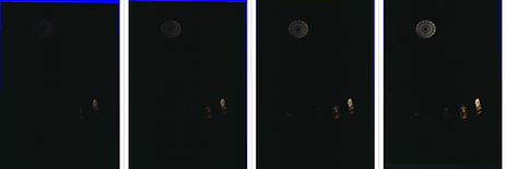
Input Different Exposure Images:


Output:
Global Tone Mapping

Local Tone Mapping

References:
The Chinese University of Hong Kong
Course CSCI3290 - Computational Photography
Prof. Jia Jia Yia